Getting started with Hyrax

Installation

Hyrax can be installed via pip:

pip install hyrax

Hyrax is officially supported and tested with Python versions 3.10, 3.11, 3.12, and 3.13. Other versions may work but are not guaranteed to be compatible.

We strongly encourage the use of a virtual environment when working with Hyrax because Hyrax depends on several open source packages that may have conflicting dependencies with other packages you have installed.

First Steps

This getting started example uses Hyrax to train a small convolutional neural network to classify CIFAR data. It is based on a similar PyTorch tutorial. We also use the CIFAR10 dataset: Learning multiple layers of features from tiny images. Alex Krizhevsky, 2009.

As part of this example we will:

1. Create a Hyrax instance

2. Specify a model and a dataset

3. Train the model

4. Predict with the model

5. Evaluate the results

Create a hyrax instance

The main driver for Hyrax is the Hyrax class. To get started we’ll create an instance of this class.

from hyrax import Hyrax

h = Hyrax()

When we create the Hyrax instance, it will automatically load a default configuration file. This file contains default settings for all of the components that Hyrax uses.

Specify a model

We’ll need to let Hyrax know which model to use for training. Here we’ll tell Hyrax to use the built-in HyraxCNN model that is based on the simple CNN architecture from the PyTorch CIFAR10 tutorial.

h.set_config('model.name', 'HyraxCNN')

Defining the dataset

We’ll also need to tell Hyrax what data should be used for training, in this case the CIFAR10 dataset. Hyrax has a built in dataset class for working with CIFAR10 data, so we’ll configure that here. You can learn more about the CIFAR10 at the offical site: https://www.cs.toronto.edu/~kriz/cifar.html

model_inputs_definition = {
     "train": {
         "data": {
             "dataset_class": "HyraxCifarDataset",
             "data_location": "./data",
             "fields": ["image", "label"],
             "primary_id_field": "object_id",
         },
     }
 }

 h.set_config("model_inputs", model_inputs_definition)

This may appear overwhelming, especially for a simple case, but being explicit about the dataset configuration will allow for great flexibility down the line when working with more complex data.

Training the model

Now that we have the model and data specified, we’re ready for training. We’ll use the train verb to kick off the training process.

h.train()

Once the training is complete, the model weights will be saved in a timestamped directory with a name similar to /YYYYmmdd-HHMMSS-train-RAND. Note that RAND is a random four character string to avoid collisions if you run multiple training sessions in the same second.

Predicting with the model

Now that we’ve trained a model, we can use it to infer classes of samples from the CIFAR10 test dataset. First we’ll add to our model input definition to specify the data to use for inference.

model_inputs_definition["infer"] = {
    "data": {
        "dataset_class": "HyraxCifarDataset",
        "data_location": "./data",
        "fields": ["image"],
        "primary_id_field": "object_id",
        "dataset_config": {
            "use_training_data": False,
        },
    },
}

h.set_config("model_inputs", model_inputs_definition)

Then we’ll use Hyrax’s infer verb to load the trained model weights and process the data defined above.

inference_results = h.infer()

Evaluate the performance

Let’s compare the model’s predictions to the actual labels from the test dataset. The model’s prediction is a 10 element vector where the largest value represents the highest confidence class. So we’ll extract the index of the max value for each prediction and save that as predicted_classes. We’ll also load the original test data to get the true labels for comparison.

import numpy as np
import pickle

# Accumulate the predicted classes
predicted_classes = np.zeros(len(inference_results)).astype(int)
for i, result in enumerate(inference_results):
    predicted_classes[i] = np.argmax(result["model_output"])

# Load the true labels
with open("./data/cifar-10-batches-py/test_batch", "rb") as f_in:
    test_data = pickle.load(f_in, encoding="bytes")

Using scikit-learn’s confusion_matrix, we can compute and display the confusion matrix to see how well the model performed on each class.

import matplotlib.pyplot as plt
from sklearn.metrics import ConfusionMatrixDisplay, confusion_matrix

y_true = test_data[b"labels"]
y_pred = predicted_classes.tolist()

correct = 0
for t, p in zip(y_true, y_pred):
    correct += t == p

print("\nAccuracy for test dataset:", correct / len(y_true))

cm = confusion_matrix(y_true, y_pred)
disp = ConfusionMatrixDisplay(confusion_matrix=cm)
disp.plot()
plt.show()

>> Accuracy for test dataset: 0.5003

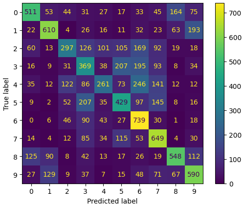
The model performs much better than chance (which would be 10%) with some classes being predicted more accurately.