Astronomy Supervised#
This example demonstrates a supervised astronomy workflow for classifying astronomical transients from their multi-band light curves.
Note: This notebook is intentionally slightly more involved than the Hello World and Astronomy Unsupervised examples. In this example, we define a custom dataset class and a custom model for 1-D light-curve data. If you are new to Hyrax, we recommend working through those earlier examples first.
Overview#
The workflow is:
Download the PLAsTiCC light-curve dataset from the Multi-Modal Universe project
Preprocess the variable-length, irregularly sampled light curves into per-observation sequences
Define a custom Hyrax dataset (with a custom collate function for variable-length padding) and a GRU-based recurrent model
Train the classifier with class-weighted loss to handle PLAsTiCC’s severe class imbalance
Predict transient classes on held-out test data
Evaluate performance with a confusion matrix
The PLAsTiCC challenge was a major Kaggle competition for photometric transient classification on simulated LSST light curves. The winning solution, AVOCADO, used Gaussian Process interpolation followed by a gradient-boosted tree. Several other top-placing teams — including the 2nd-place solution — used recurrent neural networks (GRUs and LSTMs) on the raw observation sequences.
We follow this RNN-based approach here because it maps naturally onto Hyrax’s dataset and model APIs and demonstrates how to handle variable-length, irregularly sampled time series without any interpolation or binning. GRUs process observations sequentially and encode the time gap between observations as an explicit input feature.
The data#
This example uses the PLAsTiCC training set as reformatted by the Multi-Modal Universe (MMU) project. It contains roughly 7,800 labeled light curves across 14 classes of astronomical transients and variables — including SNIa, SNII, SNIbc, TDE, AGN, RR Lyrae, kilonova, and more. Each light curve has multi-band photometry (LSST ugrizY) with irregular cadence.
The model#
We define a GRU (Gated Recurrent Unit) recurrent neural network that processes each light curve as a variable-length sequence of observations. Each observation is represented as a feature vector containing the time elapsed since the previous observation, the flux, the flux uncertainty, and a one-hot encoding of the photometric band. This approach naturally handles irregular cadence and variable-length sequences — unlike a CNN, the GRU does not require binning or interpolation, so no temporal information is lost.
Install dependencies#
We need Hyrax and the HuggingFace datasets library to download the MMU data. You can skip this step if these are already installed in your environment.
[ ]:
%pip install datasets
Download the PLAsTiCC dataset#
We load the PLAsTiCC training set directly from the MMU HuggingFace repository. The download is roughly 15 MB.
[2]:
from datasets import load_dataset

ds = load_dataset("MultimodalUniverse/plasticc", split="train")

print(f"Loaded {len(ds)} samples")
print(f"\nFeatures: {list(ds.features.keys())}")
print(f"\nFirst sample keys: {list(ds[0].keys())}")
print(f"Light curve keys:  {list(ds[0]['lightcurve'].keys())}")
Loaded 7848 samples

Features: ['lightcurve', 'hostgal_photoz', 'hostgal_specz', 'redshift', 'obj_type', 'object_id']

First sample keys: ['lightcurve', 'hostgal_photoz', 'hostgal_specz', 'redshift', 'obj_type', 'object_id']
Light curve keys:  ['band', 'flux', 'flux_err', 'time']
Preprocess light curves#
The raw light curves have variable lengths and irregular cadence across six LSST bands. Instead of binning into a fixed grid (which destroys temporal structure), we keep every observation and represent it as a feature vector that a recurrent model can consume directly.
For each object we:
Filter out zero-padded placeholder observations
Sort all observations chronologically (across all bands)
Compute the time elapsed since the previous observation (delta-t)
Normalize flux per object
One-hot encode the photometric band
This produces a variable-length sequence of 9-dimensional feature vectors per object: (delta_t, flux, flux_err, u, g, r, i, z, Y).
[3]:
import numpy as np
from pathlib import Path

# LSST band names in wavelength order → channel indices
BAND_TO_IDX = {"u": 0, "g": 1, "r": 2, "i": 3, "z": 4, "Y": 5}
NUM_BANDS = len(BAND_TO_IDX)
INPUT_DIM = 1 + 1 + 1 + NUM_BANDS  # delta_t, flux, flux_err, 6 band one-hots = 9


def extract_sequence(lc):
    """Convert a variable-length multi-band light curve into a feature sequence.

    Returns an (N_obs, 9) float32 array where each row is
    (delta_t, flux, flux_err, u, g, r, i, z, Y).
    """
    band_strs = np.asarray(lc["band"])
    times = np.asarray(lc["time"], dtype=np.float64)
    fluxes = np.asarray(lc["flux"], dtype=np.float32)
    flux_errs = np.asarray(lc["flux_err"], dtype=np.float32)

    # The MMU PLAsTiCC format zero-pads unused observation slots.
    real = (times > 0) | (fluxes != 0)
    band_strs, times, fluxes, flux_errs = (
        band_strs[real],
        times[real],
        fluxes[real],
        flux_errs[real],
    )

    if len(times) == 0:
        return np.zeros((1, INPUT_DIM), dtype=np.float32)

    # Sort chronologically
    order = np.argsort(times)
    band_strs, times, fluxes, flux_errs = (
        band_strs[order],
        times[order],
        fluxes[order],
        flux_errs[order],
    )

    # Delta-t: time since previous observation (first obs gets 0)
    delta_t = np.zeros(len(times), dtype=np.float32)
    delta_t[1:] = np.diff(times).astype(np.float32)
    # Normalize delta_t to [0, 1]
    dt_max = delta_t.max()
    if dt_max > 0:
        delta_t /= dt_max

    # Normalize flux per object
    max_abs = np.abs(fluxes).max()
    if max_abs > 0:
        fluxes /= max_abs
        flux_errs /= max_abs

    # One-hot band encoding
    band_onehot = np.zeros((len(times), NUM_BANDS), dtype=np.float32)
    for j, bs in enumerate(band_strs):
        idx = BAND_TO_IDX.get(str(bs), -1)
        if idx >= 0:
            band_onehot[j, idx] = 1.0

    # Stack into (N_obs, 9) feature matrix
    seq = np.column_stack([delta_t, fluxes, flux_errs, band_onehot])
    return seq.astype(np.float32)


# --- Process every sample ---
all_seqs, all_raw_labels = [], []
for sample in ds:
    all_seqs.append(extract_sequence(sample["lightcurve"]))
    all_raw_labels.append(sample["obj_type"])

# Map string labels to contiguous integers
unique_classes = sorted(set(all_raw_labels))
label_to_idx = {c: i for i, c in enumerate(unique_classes)}
idx_to_name = {i: c for i, c in enumerate(unique_classes)}
labels = np.array([label_to_idx[l] for l in all_raw_labels])

seq_lengths = [len(s) for s in all_seqs]
print(f"Preprocessed {len(all_seqs)} light curves")
print(
    f"Sequence lengths: min={min(seq_lengths)}, median={int(np.median(seq_lengths))}, max={max(seq_lengths)}"
)
print(f"Feature dim: {INPUT_DIM}")
print(f"\nClasses: {len(unique_classes)}")
for i, name in idx_to_name.items():
    count = (labels == i).sum()
    print(f"  {i:>2d}: {name} ({count} samples)")

# --- Compute class weights (inverse frequency) for weighted loss ---
class_counts = np.bincount(labels)
class_weights = len(labels) / (len(unique_classes) * class_counts)
class_weights = class_weights.astype(np.float32)
print(f"\nClass weights: {dict(zip(idx_to_name.values(), class_weights.round(2)))}")

# --- 80/20 stratified train/test split ---
from sklearn.model_selection import train_test_split

train_idx, test_idx = train_test_split(
    np.arange(len(labels)),
    test_size=0.2,
    random_state=42,
    stratify=labels,
)

data_dir = Path("./data/plasticc")
data_dir.mkdir(parents=True, exist_ok=True)

# Save sequences as object arrays (variable length) + labels + class weights
np.savez(
    data_dir / "train.npz",
    sequences=np.array([all_seqs[i] for i in train_idx], dtype=object),
    labels=labels[train_idx],
    object_ids=train_idx,
    class_weights=class_weights,
)
np.savez(
    data_dir / "test.npz",
    sequences=np.array([all_seqs[i] for i in test_idx], dtype=object),
    labels=labels[test_idx],
    object_ids=test_idx,
)

print(f"\nSaved {len(train_idx)} train / {len(test_idx)} test samples to {data_dir}")
Preprocessed 7848 light curves
Sequence lengths: min=34, median=100, max=296
Feature dim: 9

Classes: 14
   0: AGN (370 samples)
   1: EB (924 samples)
   2: KN (102 samples)
   3: M-dwarf (981 samples)
   4: MicroLens-Single (151 samples)
   5: Mira (30 samples)
   6: RRL (239 samples)
   7: SLSN-I (175 samples)
   8: SNII (1193 samples)
   9: SNIa (2313 samples)
  10: SNIa-91bg (208 samples)
  11: SNIax (183 samples)
  12: SNIbc (484 samples)
  13: TDE (495 samples)

Class weights: {'AGN': np.float32(1.52), 'EB': np.float32(0.61), 'KN': np.float32(5.5), 'M-dwarf': np.float32(0.57), 'MicroLens-Single': np.float32(3.71), 'Mira': np.float32(18.69), 'RRL': np.float32(2.35), 'SLSN-I': np.float32(3.2), 'SNII': np.float32(0.47), 'SNIa': np.float32(0.24), 'SNIa-91bg': np.float32(2.7), 'SNIax': np.float32(3.06), 'SNIbc': np.float32(1.16), 'TDE': np.float32(1.13)}

Saved 6278 train / 1570 test samples to data/plasticc

Saved 6278 train / 1570 test samples to data/plasticc
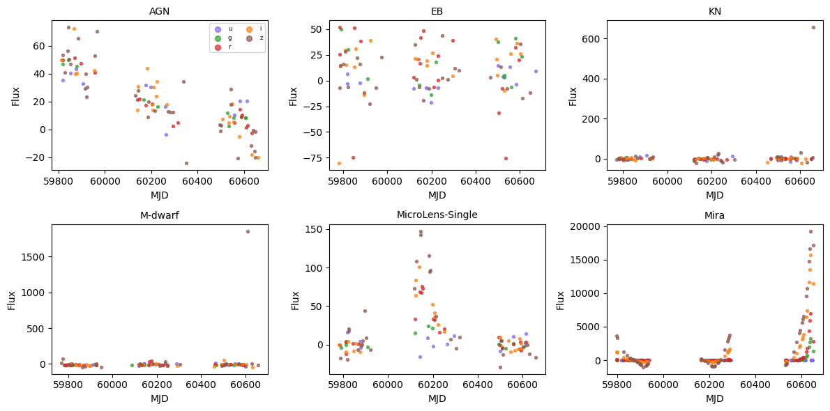
Let’s visualize a few example light-curve sequences. Each point is a single observation, colored by band, and plotted at its actual observation time — no binning or interpolation.
[4]:
import matplotlib.pyplot as plt

BAND_NAMES = list(BAND_TO_IDX.keys())
band_colors = {"u": "#7B68EE", "g": "#2ca02c", "r": "#d62728", "i": "#ff7f0e", "z": "#8c564b", "Y": "#1f77b4"}

show_classes = list(range(min(6, len(idx_to_name))))
fig, axes = plt.subplots(2, 3, figsize=(12, 6))

for ax, cls in zip(axes.flat, show_classes):
    sample_idx = np.where(labels == cls)[0][0]
    lc = ds[int(sample_idx)]["lightcurve"]

    band_strs = np.asarray(lc["band"])
    times = np.asarray(lc["time"], dtype=np.float64)
    fluxes = np.asarray(lc["flux"], dtype=np.float32)
    real = (times > 0) | (fluxes != 0)

    for band_name in BAND_NAMES:
        mask = real & (band_strs == band_name)
        if mask.any():
            ax.scatter(
                times[mask],
                fluxes[mask],
                label=band_name,
                c=band_colors[band_name],
                s=8,
                alpha=0.7,
            )
    ax.set_title(idx_to_name[cls], fontsize=10)
    ax.set_xlabel("MJD")
    ax.set_ylabel("Flux")

axes[0, 0].legend(fontsize=6, ncol=2, markerscale=2)
plt.tight_layout()
plt.show()
Define a custom dataset#
To use preprocessed data with Hyrax we subclass HyraxDataset. A dataset needs to implement:
__len__— the number of samplesget_<field>(idx)methods for each field the model will consume
Because our light-curve sequences have variable lengths, we also define a collate method. Hyrax automatically detects this method and uses it instead of the default numpy-stacking collation. Our collate pads all sequences in a batch to the same length and returns the true sequence lengths so the model can use pack_padded_sequence.
Note: The dataset class below uses
.get()with inline defaults to keep this notebook concise. In practice, we discourage this pattern because it scatters default values across your code instead of keeping them in one place. Instead, define your defaults in a TOML configuration file and access config values with direct[]lookups. See the Configuration System documentation for details.
[5]:
from hyrax.datasets import HyraxDataset


class PLAsTiCCSequenceDataset(HyraxDataset):
    """Hyrax dataset for variable-length PLAsTiCC light-curve sequences."""

    def __init__(self, config: dict, data_location=None):
        data_dir = Path(data_location)

        # Pick train or test split based on config
        ds_config = config.get("data_set", {}).get("PLAsTiCCSequenceDataset", {})
        split = "train" if ds_config.get("use_training_data", True) else "test"

        data = np.load(data_dir / f"{split}.npz", allow_pickle=True)
        self.sequences = data["sequences"]  # object array of (seq_len, 9) arrays
        self.labels = data["labels"]
        self.object_ids = data["object_ids"]

        # Store class weights if available (training split only)
        self.class_weights = data["class_weights"] if "class_weights" in data else None

        super().__init__(config)

    def get_sequence(self, idx):
        """Return the feature sequence for one object — shape (seq_len, 9)."""
        return np.array(self.sequences[idx], dtype=np.float32)

    def get_label(self, idx):
        """Return the integer class label."""
        return int(self.labels[idx])

    def get_object_id(self, idx):
        """Return a unique string identifier."""
        return str(self.object_ids[idx])

    def __len__(self):
        return len(self.labels)

    def collate(self, samples: list[dict]) -> dict:
        """Pad variable-length sequences to the max length in the batch.

        Parameters
        ----------
        samples
            List of dicts, each with keys like ``"sequence"`` and ``"label"``.

        Returns
        -------
        dict
            ``"sequence"`` — float32 array (batch, max_len, 9), zero-padded
            ``"label"`` — int64 array (batch,)
            ``"lengths"`` — int64 array (batch,) with true sequence lengths
        """
        result = {}

        # Sequences require padding — only process if present in this batch
        if "sequence" in samples[0]:
            seqs = [s["sequence"] for s in samples]
            lengths = np.array([len(s) for s in seqs], dtype=np.int64)
            max_len = int(lengths.max())

            padded = np.zeros((len(seqs), max_len, seqs[0].shape[-1]), dtype=np.float32)
            for i, s in enumerate(seqs):
                padded[i, : len(s)] = s

            result["sequence"] = padded
            result["lengths"] = lengths

        # Labels are present during training but not inference
        if "label" in samples[0]:
            result["label"] = np.array([s["label"] for s in samples], dtype=np.int64)

        return result
Define a custom model#
We use a bidirectional GRU that processes the padded observation sequences using PyTorch’s pack_padded_sequence / pad_packed_sequence to efficiently skip padding positions. The final hidden states from both directions are concatenated and passed through a classification head.
The model also sets its own loss function (self.criterion) with class weights computed from the training data. Hyrax’s @hyrax_model decorator detects this and uses it instead of loading a criterion from the config.
Note: As with the dataset class, the model below uses
.get()with inline defaults for brevity. In your own projects, define these defaults in a TOML config file and use direct[]access. See the Configuration System documentation.
[6]:
import torch
import torch.nn as nn
from torch.nn.utils.rnn import pack_padded_sequence, pad_packed_sequence
from hyrax.models import hyrax_model


@hyrax_model
class LightCurveGRU(nn.Module):
    """A bidirectional GRU for variable-length multi-band light-curve classification."""

    def __init__(self, config, data_sample=None):
        super().__init__()
        self.config = config
        model_config = config["model"]["LightCurveGRU"]

        input_dim = model_config.get("input_dim", INPUT_DIM)
        hidden_size = model_config.get("hidden_size", 128)
        num_layers = model_config.get("num_layers", 2)
        dropout = model_config.get("dropout", 0.3)
        num_classes = model_config["output_classes"]
        self.grad_clip = model_config.get("grad_clip", 1.0)

        self.gru = nn.GRU(
            input_size=input_dim,
            hidden_size=hidden_size,
            num_layers=num_layers,
            batch_first=True,
            bidirectional=True,
            dropout=dropout if num_layers > 1 else 0.0,
        )
        # Bidirectional → 2x hidden_size
        self.classifier = nn.Sequential(
            nn.Dropout(dropout),
            nn.Linear(hidden_size * 2, 64),
            nn.ReLU(),
            nn.Dropout(dropout),
            nn.Linear(64, num_classes),
        )

        # Set class-weighted loss before @hyrax_model wiring runs
        cw = model_config.get("class_weights", None)
        if cw is not None:
            weight = torch.tensor(cw, dtype=torch.float32)
            self.criterion = nn.CrossEntropyLoss(weight=weight)

    def forward(self, x):
        sequences, labels, lengths = x

        # pack_padded_sequence needs lengths on CPU
        lengths_cpu = lengths.cpu()

        packed = pack_padded_sequence(
            sequences,
            lengths_cpu,
            batch_first=True,
            enforce_sorted=False,
        )
        _, hidden = self.gru(packed)
        # hidden shape: (num_layers * 2, batch, hidden_size)
        # Concatenate final forward and backward hidden states
        fwd = hidden[-2]  # last layer, forward
        bwd = hidden[-1]  # last layer, backward
        combined = torch.cat([fwd, bwd], dim=-1)  # (batch, hidden_size * 2)

        return self.classifier(combined)

    def train_batch(self, batch):
        _, labels, _ = batch
        self.optimizer.zero_grad()
        outputs = self(batch)
        loss = self.criterion(outputs, labels)
        loss.backward()
        nn.utils.clip_grad_norm_(self.parameters(), self.grad_clip)
        self.optimizer.step()
        return {"loss": loss.item()}

    def validate_batch(self, batch):
        _, labels, _ = batch
        outputs = self(batch)
        loss = self.criterion(outputs, labels)
        return {"loss": loss.item()}

    def test_batch(self, batch):
        return self.validate_batch(batch)

    def infer_batch(self, batch):
        return self(batch)

    @staticmethod
    def prepare_inputs(data_dict):
        """Convert the collated data dictionary to numpy arrays."""
        import numpy as np

        data = data_dict["data"]
        sequence = np.asarray(data["sequence"], dtype=np.float32)
        lengths = np.asarray(data["lengths"], dtype=np.int64)
        label = np.asarray(data.get("label", np.zeros(len(lengths))), dtype=np.int64)
        return (sequence, label, lengths)
Initialize Hyrax and configure#
From here the workflow is the same as any other Hyrax example: create a Hyrax instance, point it at our custom model and dataset, and run verbs.
[ ]:
from hyrax import Hyrax

h = Hyrax()

h.set_config("model.name", "LightCurveGRU")

# Create the config section for our custom model. We pass the class weights
# so the model can build a weighted CrossEntropyLoss in its __init__.
h.config["model"]["LightCurveGRU"] = {
    "output_classes": len(idx_to_name),
    "input_dim": INPUT_DIM,
    "hidden_size": 256,
    "num_layers": 2,
    "dropout": 0.3,
    "grad_clip": 1.0,
    "class_weights": class_weights.tolist(),
}

# Adam is the standard optimizer for RNNs — SGD struggles with recurrent gradients
h.set_config("optimizer.name", "torch.optim.Adam")
h.config["torch.optim.Adam"] = {"lr": 1e-3}

h.set_config("data_loader.batch_size", 64)
h.set_config("train.epochs", 50)
Define the dataset and train#
We configure the data_request to use our custom PLAsTiCCSequenceDataset and request the sequence and label fields. Note how the field names match the get_sequence and get_label methods we defined above. Because our dataset defines a collate method, Hyrax will automatically use it to pad variable-length sequences in each batch.
[ ]:
data_request_definition = {
    "train": {
        "data": {
            "dataset_class": "PLAsTiCCSequenceDataset",
            "data_location": "./data/plasticc",
            "fields": ["sequence", "label"],
            "primary_id_field": "object_id",
            "split_fraction": 1.0,
        },
    },
}

h.set_config("data_request", data_request_definition)

trained_model = h.train()
[2026-03-27 23:27:30,887 hyrax.verbs.train:INFO] Finished Training
INFO  [hyrax.verbs.train] Finished Training
Predict with the model#
We now classify the held-out test light curves. Setting use_training_data to False via dataset_config tells our dataset to load test.npz instead of train.npz.
For custom datasets the dataset_config dictionary must be nested under the dataset class name so that Hyrax knows which config section to update.
[ ]:
data_request_definition["infer"] = {
    "data": {
        "dataset_class": "PLAsTiCCSequenceDataset",
        "data_location": "./data/plasticc",
        "fields": ["sequence", "object_id"],
        "primary_id_field": "object_id",
        "dataset_config": {
            "PLAsTiCCSequenceDataset": {
                "use_training_data": False,
            },
        },
    },
}

h.set_config("data_request", data_request_definition)

inference_results = h.infer()
[2026-03-27 23:27:31,039 hyrax.models.model_utils:INFO] Updated config['infer']['model_weights_file'] to: /mmfs1/gscratch/dirac/aritrag/repos/hyrax/docs/pre_executed/results/20260327-232400-train-QJlv/example_model.pth
INFO  [hyrax.models.model_utils] Updated config['infer']['model_weights_file'] to: /mmfs1/gscratch/dirac/aritrag/repos/hyrax/docs/pre_executed/results/20260327-232400-train-QJlv/example_model.pth
[2026-03-27 23:27:31,042 hyrax.verbs.infer:INFO] Saving inference results at: /mmfs1/gscratch/dirac/aritrag/repos/hyrax/docs/pre_executed/results/20260327-232730-infer-7AlE
INFO  [hyrax.verbs.infer] Saving inference results at: /mmfs1/gscratch/dirac/aritrag/repos/hyrax/docs/pre_executed/results/20260327-232730-infer-7AlE
[2026-03-28T06:27:31Z WARN  lance::dataset::write::insert] No existing dataset at /mmfs1/gscratch/dirac/aritrag/repos/hyrax/docs/pre_executed/results/20260327-232730-infer-7AlE/lance_db/results.lance, it will be created
[2026-03-27 23:27:31,851 hyrax.pytorch_ignite:INFO] Total evaluation time: 0.79[s]
INFO  [hyrax.pytorch_ignite] Total evaluation time: 0.79[s]
[2026-03-27 23:27:31,852 hyrax.datasets.result_dataset:INFO] Optimizing Lance table after 25 batches
INFO  [hyrax.datasets.result_dataset] Optimizing Lance table after 25 batches
[2026-03-27 23:27:31,876 hyrax.datasets.result_dataset:INFO] Lance table optimization complete
INFO  [hyrax.datasets.result_dataset] Lance table optimization complete
[2026-03-27 23:27:31,877 hyrax.verbs.infer:INFO] Inference Complete.
INFO  [hyrax.verbs.infer] Inference Complete.
Evaluate the performance#
The model outputs a 14-element vector per light curve. The index of the maximum value is the predicted class. We compare against the true labels and display a confusion matrix.
[10]:
import matplotlib.pyplot as plt
from sklearn.metrics import ConfusionMatrixDisplay, confusion_matrix

# Predicted classes
y_pred = [inference_results[i].argmax() for i in range(len(inference_results))]

# True labels from saved test split
test_data = np.load("./data/plasticc/test.npz")
y_true = test_data["labels"].tolist()

correct = sum(t == p for t, p in zip(y_true, y_pred))
print(f"Accuracy: {correct / len(y_true):.2%}")

class_names = [idx_to_name[i] for i in range(len(idx_to_name))]

cm = confusion_matrix(y_true, y_pred)
fig, ax = plt.subplots(figsize=(10, 8))
disp = ConfusionMatrixDisplay(confusion_matrix=cm, display_labels=class_names)
disp.plot(ax=ax, xticks_rotation=45, values_format="d")
plt.tight_layout()
plt.show()
Accuracy: 69.68%
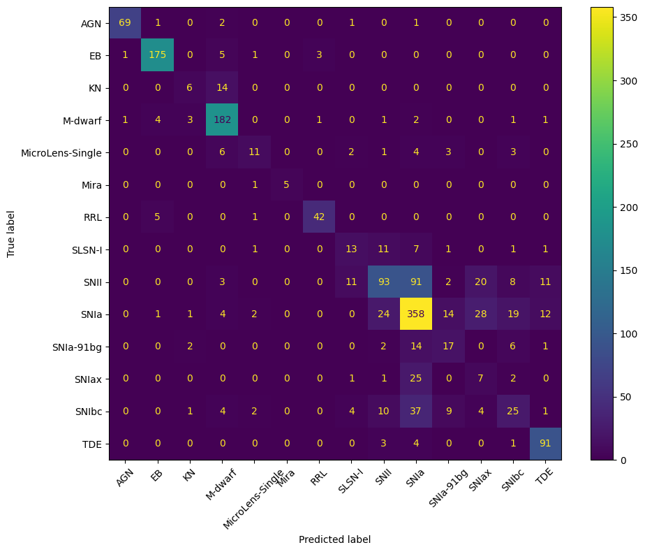
The GRU achieves roughly 70% accuracy on 14 classes; but the PLAsTiCC Kaggle competition winners achieved much higher performance by combining Gaussian Process interpolation, hand-crafted features, and gradient-boosted trees. The goal of this notebook is not to compete with those results, but to show how Hyrax’s model and dataset APIs can be used to build a recurrent classifier from scratch on time-series data.
What to take away#
Hyrax is not limited to images. By defining a custom dataset and model, you can work with light curves, spectra, or any other data modality.
Custom datasets subclass
HyraxDatasetand provideget_<field>()methods. For variable-length data, define acollatemethod — Hyrax will detect and use it automatically.Custom models are standard
torch.nn.Moduleclasses decorated with@hyrax_model. Implementtrain_batch,infer_batch, andprepare_inputs, and Hyrax handles the rest. You can setself.criteriondirectly in__init__to use a custom loss (e.g., class-weighted).The core Hyrax workflow is the same regardless of data type: configure → train → infer → evaluate.
[ ]: