Creating and Querying a Vector Database

A vector database enables efficient similarity searches over latent representations. In this notebook we train a model, run inference to produce vectors, store them in a vector database, and query for nearest neighbors.

First, create a Hyrax object, configure it to train the default HyraxAutoencoderV2 model on CIFAR-10 data, then run infer to produce encoded vectors.

from hyrax import Hyrax

h = Hyrax()
h.config["model"]["name"] = "HyraxAutoencoderV2"

data_request = {
    "train": {
        "data": {
            "dataset_class": "HyraxCifarDataset",
            "data_location": "./data",
            "fields": ["image"],
            "primary_id_field": "object_id",
            "split_fraction": 1.0,
        },
    },
}
h.set_config("data_request", data_request)

h.config["train"]["epochs"] = 10
model = h.train()

data_request = {
    "infer": {
        "data": {
            "dataset_class": "HyraxCifarDataset",
            "data_location": "./data",
            "fields": ["image", "object_id"],
            "primary_id_field": "object_id",
            "dataset_config": {
                "HyraxCifarDataset": {
                    "use_training_data": False,
                },
            },
        },
    },
}
h.set_config("data_request", data_request)

h.infer()

Choosing a Vector Database Backend

Hyrax supports two vector database backends: ChromaDB (default) and Qdrant. The backend is selected via h.config["vector_db"]["name"] and must be set before calling h.save_to_database() or h.database_connection().

Each backend has its own sub-section in the config for backend-specific settings. For Qdrant, vector_size must be set to match your model’s latent dimension.

# Use ChromaDB (default):
h.config["vector_db"]["name"] = "chromadb"

# To switch to Qdrant instead, comment out the line above and uncomment these:
# h.config["vector_db"]["name"] = "qdrant"
# h.config["vector_db"]["qdrant"]["vector_size"] = 64  # qdrant database requires specifying the latent dimension

print(f"Using vector database backend: {h.config['vector_db']['name']}")

Using vector database backend: chromadb

Creating the Database

Now populate the vector database with the inference results. By default h.save_to_database() uses the most recent infer output and creates a new timestamped directory — both can be overridden:

h.save_to_database([input_dir="/path/to/input",] [output_dir="/path/to/output"])

Note: To add more data to an existing database, pass the existing database directory as output_dir.

print(f"Filling a {h.config['vector_db']['name']} database with the results of inference.")
h.save_to_database()

Filling a chromadb database with the results of inference.

[2026-03-06 10:43:25,614 hyrax.verbs.save_to_database:INFO] Saving vector database at /home/drew/code/hyrax/docs/pre_executed/results/20260306-104325-vector-db-nrKM
100%|██████████| 20/20 [00:18<00:00,  1.09it/s]
[2026-03-06 10:43:44,097 hyrax.verbs.save_to_database:INFO] Vector database insertion complete. Total time: 1.856s for 20 batches

Querying the Database

Now that the vector database has been populated, it can be used for similarity search. First we’ll need to establish a connection using h.database_connection(). By default h.database_connection() will connect to the most recently created database. Use h.database_connection(database_dir=<path_to_database>) to connect to a specific database.

With the connection established, we have access to three types of queries:

• get_by_id to retrieve the vector associated with a particular id

• search_by_id to retrieve the k nearest neighbors to a particular id

• search_by_vector to retrieve the k nearest neighbors to a particular input vector

conn = h.database_connection()

get_by_id

With get_by_id we can retrieve the vectors associated with some ids. The result is a dictionary where the keys are id strings and values are the numpy array vectors retrieved from the database.

results = conn.get_by_id(ids=["00334", "09598", "04493"])

for k, v in results.items():
    print(f"Id: {k}, Vector: {v}")

Id: 00334, Vector: [-0.00633008 -0.001161    0.01861886  0.00101888  0.03130957 -0.02134504
 -0.01874688  0.00044905 -0.02996075  0.01360556  0.01252521  0.02144271
  0.0141634  -0.0076211  -0.01682794  0.02824579  0.00716362 -0.03539264
  0.01784317  0.00433305  0.03272513  0.00211681  0.00532972 -0.01692898
  0.01164115  0.01477985  0.02368246  0.02142361  0.02833303 -0.01588214
 -0.00331219  0.01074693  0.02021811 -0.01372821  0.00634572 -0.01904588
 -0.04155122 -0.00031589 -0.02161333 -0.02701451  0.0160961  -0.02697142
  0.0256546  -0.01524267  0.00349341 -0.02677254  0.03321952 -0.02817712
  0.00225346  0.0262328  -0.00848513  0.01849484  0.01200403  0.01364053
 -0.00101044  0.01686103 -0.02717537 -0.01816413  0.02594164  0.00684086
  0.00868795  0.0334354  -0.00548371  0.01636631]
Id: 04493, Vector: [-0.00595091 -0.00154015  0.01865609  0.0010969   0.03096601 -0.02165768
 -0.0191785   0.00018299 -0.03005512  0.01375524  0.01234648  0.02179527
  0.01459047 -0.00785387 -0.01675942  0.02804837  0.00676632 -0.03539746
  0.01758233  0.0039999   0.0329616   0.00213138  0.00538168 -0.01684992
  0.01126629  0.01481402  0.0235731   0.02136657  0.0285771  -0.01606328
 -0.00341822  0.01031781  0.02009598 -0.01387708  0.00641984 -0.01879212
 -0.04140575 -0.00019975 -0.02180372 -0.02692492  0.01640445 -0.02741425
  0.02583189 -0.01507939  0.00393042 -0.02705386  0.03342287 -0.02855648
  0.00175818  0.02644471 -0.00835482  0.01838988  0.0119083   0.01366867
 -0.0008908   0.01700609 -0.02721358 -0.01794845  0.02616784  0.00698005
  0.00919942  0.0331492  -0.00568041  0.01626557]
Id: 09598, Vector: [-6.22524135e-03 -1.34877255e-03  1.86340008e-02  1.57952262e-03
  3.07085328e-02 -2.20955070e-02 -1.93371549e-02  4.31667460e-04
 -3.04584503e-02  1.37488693e-02  1.18468907e-02  2.15803888e-02
  1.44278044e-02 -9.06416588e-03 -1.68876238e-02  2.86653619e-02
  6.76234160e-03 -3.51960063e-02  1.75719652e-02  3.67353018e-03
  3.23572308e-02  1.81757612e-03  5.86301181e-03 -1.73177980e-02
  1.01112444e-02  1.54122068e-02  2.29081400e-02  2.15121433e-02
  2.91775167e-02 -1.61609389e-02 -3.23996786e-03  1.05957631e-02
  2.03442127e-02 -1.38517637e-02  6.49915682e-03 -1.92545746e-02
 -4.10405584e-02 -3.99870332e-05 -2.22808756e-02 -2.73416378e-02
  1.61282644e-02 -2.71060374e-02  2.54529901e-02 -1.54343611e-02
  3.68494052e-03 -2.67027617e-02  3.30936760e-02 -2.86820810e-02
  2.01753806e-03  2.63735838e-02 -8.28913413e-03  1.81108173e-02
  1.19146770e-02  1.33302826e-02 -8.25810246e-04  1.61902625e-02
 -2.70545240e-02 -1.73545554e-02  2.63042618e-02  5.65342605e-03
  9.47053544e-03  3.26765366e-02 -5.33952937e-03  1.61481202e-02]

search_by_id

Now we’ll search for nearest neighbors. First we search for the k nearest neighbors of using an id from the database. Note that the closest of the 5 neighbors is the vector itself, since it’s in the database. The returned dictionary contains the ids of the nearest neighbors in order of increasing distance.

conn.search_by_id("04493", k=5)

{'04493': ['04493', '04184', '01724', '01325', '03790']}

search_by_vector

We can also search using a raw vector. Here we reuse the vector retrieved by get_by_id, so the results should match the previous search_by_id call. The input is a list of vectors — they don’t need to come from the database (e.g. a fresh infer result works too) — so the returned dictionary is keyed by the index of each input vector.

neighbors = conn.search_by_vector([results["00334"], results["09598"], results["04493"]], k=5)
neighbors

{0: ['00334', '04493', '04473', '01308', '03120'],
 1: ['09598', '01491', '03726', '06260', '06934'],
 2: ['04493', '04184', '01724', '01325', '03790']}

Check the Results

Let’s visualize the nearest neighbors. First we get an interactive copy of the original dataset and define a couple of plotting helpers.

data_request["infer"]["data"]["fields"] = ["image", "label", "object_id"]
h.config["data_request"] = data_request
datasets = h.prepare()
dataset = datasets["infer"]

[2026-03-06 10:57:42,160 hyrax.prepare:INFO] Finished Prepare

The following is some boilerplate code for displaying either a single image or a collection of images from dataset.

import numpy as np
from matplotlib import pyplot as plt


def show_image(data):
    image = data["data"]["image"]
    title = f"Label: {data['data']['label']}, Id: {data['object_id']}"
    image = np.transpose(image, (1, 2, 0))
    min_val = np.min(image)
    max_val = np.max(image)
    image = (image - min_val) / (max_val - min_val)
    plt.imshow(image)
    if title:
        plt.title(title)
    plt.axis("off")
    plt.show()


def show_image_grid(data_list):
    rows = int(len(data_list) / 4)
    if len(data_list) % 4 != 0:
        rows += 1
    cols = 4
    if rows == 1:
        cols = len(data_list)
    fig, axes = plt.subplots(rows, cols, figsize=(cols * 3, rows * 3))
    axes = axes.flatten()

    for ax, data in zip(axes, data_list):
        image = data["data"]["image"]
        title = f"Label: {data['data'].get('label', 'N/A')}, Id: {data.get('object_id', 'N/A')}"
        image = np.transpose(image, (1, 2, 0))
        min_val = np.min(image)
        max_val = np.max(image)
        image = (image - min_val) / (max_val - min_val)
        ax.imshow(image)
        ax.set_title(title)
        ax.axis("off")

    for ax in axes[len(data_list) :]:
        ax.axis("off")

    plt.tight_layout()
    plt.show()

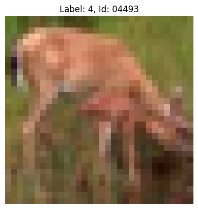
First we’ll display the image that we used for searching.

show_image(dataset[4493])

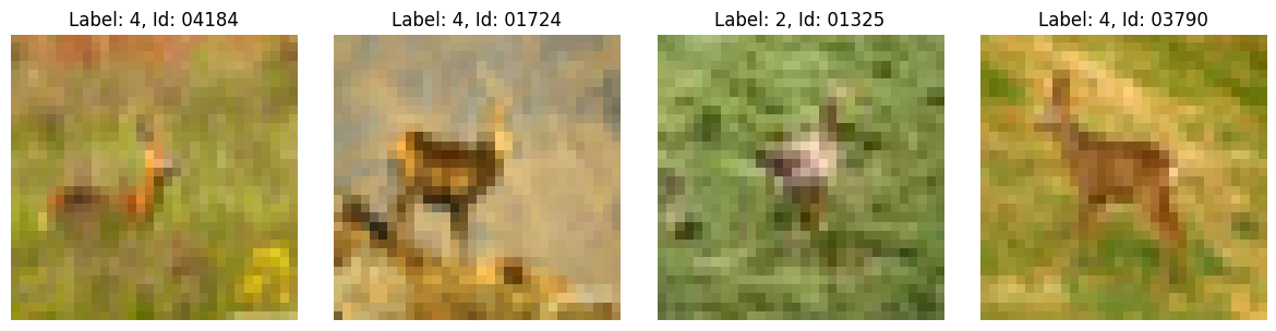
Now we’ll display the 4 nearest neighbors that retrieved from the vector database.

data_list = [dataset[int(n)] for n in neighbors[2][1:]]
show_image_grid(data_list)