Hyrax Hello World

This example walks through a small end-to-end Hyrax workflow using a built-in convolutional neural network. This page uses CIFAR10 data rather than astronomy data so that the basic Hyrax workflow is easier to see and understand. The example is based in part on the PyTorch CIFAR10 tutorial and uses the CIFAR10 dataset described in Learning multiple layers of features from tiny images, Alex Krizhevsky, 2009.

Note

In Hyrax, the basic pattern is to first create a Hyrax object, configure a model and a data_request, and then run verbs such as train and infer.

This example will:

1. Create a Hyrax instance

2. Specify a model and a dataset

3. Train the model

4. Predict with the model

5. Evaluate the results

You can also run this example in Google Colab:

Create a Hyrax instance

The main driver for Hyrax is the Hyrax class. To get started we’ll create an instance of this class.

from hyrax import Hyrax

h = Hyrax()

When we create the Hyrax instance, it automatically loads a default configuration file containing baseline settings for the components Hyrax uses. In this example, we will update configuration values directly in Python with h.set_config(...), but configuration can also be supplied in an external TOML file with entries such as model.name = "HyraxCNN". You can read more about this in the configuration system.

Specify a model

We’ll need to let Hyrax know which model to use for training. Here we’ll tell Hyrax to use the built-in HyraxCNN model that is based on the simple CNN architecture from the PyTorch CIFAR10 tutorial.

h.set_config('model.name', 'HyraxCNN')

In Hyrax terms, specifying the model is one of the required inputs for a run.

You do not need to use a built-in model. Hyrax also supports defining custom models.

Define the dataset

We’ll also need to tell Hyrax what data should be used for training, in this case the CIFAR10 dataset.

Hyrax has a built-in dataset class for working with CIFAR10 data, so we’ll configure that here. You can learn more about CIFAR10 at the official site: https://www.cs.toronto.edu/~kriz/cifar.html

data_request_definition = {
     "train": {
         "data": {
             "dataset_class": "HyraxCifarDataset",
             "data_location": "./data",
             "fields": ["image", "label"],
             "primary_id_field": "object_id",
             "split_fraction": 1.0,
         },
     }
 }

 h.set_config("data_request", data_request_definition)

This may appear overwhelming, especially for a simple case, but being explicit about the dataset configuration will allow for greater flexibility when working with more complex data. In Hyrax, the data_request defines what data each stage of the workflow should use.

Hyrax also includes built-in datasets for several astronomy workflows, and users can define custom dataset classes when needed.

Train the model

Now that we have the model and data specified, we’re ready for training. We’ll use the train verb to kick off the training process.

h.train()

Once the training is complete, the model weights will be saved in a timestamped directory with a name similar to /YYYYmmdd-HHMMSS-train-RAND. Note that RAND is a random four character string to avoid collisions if you run multiple training sessions in the same second.

Predict with the model

Now that we’ve trained a model, we can use it to infer classes of samples from the CIFAR10 test dataset. This follows the same pattern as training: first update the configuration, then run the next verb.

First we’ll add to our model input definition to specify the data to use for inference.

data_request_definition["infer"] = {
    "data": {
        "dataset_class": "HyraxCifarDataset",
        "data_location": "./data",
        "fields": ["image"],
        "primary_id_field": "object_id",
        "dataset_config": {
            "HyraxCifarDataset": {
               "use_training_data": False,
            },
        },
    },
}

h.set_config("data_request", data_request_definition)

Then we’ll use Hyrax’s infer verb to load the trained model weights and process the data defined above.

inference_results = h.infer()

Evaluate the performance

Let’s compare the model’s predictions to the actual labels from the test dataset. The model’s prediction is a 10 element vector where the largest value represents the highest confidence class. So we’ll extract the index of the max value for each prediction and save that as predicted_classes. We’ll also load the original test data to get the true labels for comparison.

import numpy as np
import pickle

# Accumulate the predicted classes
predicted_classes = np.zeros(len(inference_results)).astype(int)
for i, result in enumerate(inference_results):
    predicted_classes[i] = np.argmax(result)

# Load the true labels
with open("./data/cifar-10-batches-py/test_batch", "rb") as f_in:
    test_data = pickle.load(f_in, encoding="bytes")

Using scikit-learn’s confusion_matrix, we can compute and display the confusion matrix to see how well the model performed on each class.

import matplotlib.pyplot as plt
from sklearn.metrics import ConfusionMatrixDisplay, confusion_matrix

y_true = test_data[b"labels"]
y_pred = predicted_classes.tolist()

correct = 0
for t, p in zip(y_true, y_pred):
    correct += t == p

print("\nAccuracy for test dataset:", correct / len(y_true))

cm = confusion_matrix(y_true, y_pred)
disp = ConfusionMatrixDisplay(confusion_matrix=cm)
disp.plot()
plt.show()

>> Accuracy for test dataset: 0.5003

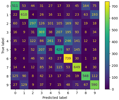
The model performs much better than chance (which would be 10%) with some classes being predicted more accurately.

What to Take Away

1. A Hyrax workflow starts by configuring a Hyrax object, which can be configured using a configuration file or updated directly in Python.

2. The model and the data_request are configured separately and are both required inputs to the workflow.

3. Verbs such as train and infer run the configured workflow.