Using a pre-trained model

Fine-tuning and transfer learning are techniques that allow a model to build on what it has already learned. Instead of starting from random weights, training begins from the weights of a prior run — often reaching lower loss in fewer epochs.

In this notebook we will:

• Train a model for a few epochs and save the weights

• Resume training from those saved weights

• Observe how the loss continues to decrease from where it left off

We’ll use the built-in HyraxCNN model with the CIFAR-10 dataset. For the first run we’ll train for only 3 epochs, leaving the model noticeably underfit, so the effect of loading pre-trained weights is easy to see.

from hyrax import Hyrax

h = Hyrax()

h.set_config("model.name", "HyraxCNN")

data_request = {
    "train": {
        "data": {
            "dataset_class": "HyraxCifarDataset",
            "data_location": "./data",
            "fields": ["image", "label"],
            "split_fraction": 0.8,
            "primary_id_field": "object_id",
        }
    },
    "validate": {
        "data": {
            "dataset_class": "HyraxCifarDataset",
            "data_location": "./data",
            "fields": ["image", "label"],
            "split_fraction": 0.2,
            "primary_id_field": "object_id",
        }
    },
}
h.set_config("data_request", data_request)

h.set_config("train.epochs", 3)

model = h.train()

Resume training from saved weights

After training, Hyrax automatically saves the model weights to the results directory. We use find_most_recent_results_dir to locate that directory, then pass the weights path to train.model_weights_file. When this setting is provided, Hyrax loads those weights before training begins rather than initializing from scratch.

We’ll also increase the number of epochs so the loss has room to fully bottom out.

from hyrax.config_utils import find_most_recent_results_dir

# Locate the directory where Hyrax saved the weights from the previous training run
results_directory = find_most_recent_results_dir(h.config, "train")

h.set_config(
    "train.model_weights_file",
    str(results_directory / "example_model.pth"),  # default filename from train.weights_filename
)

h.set_config("train.epochs", 10)
model = h.train()

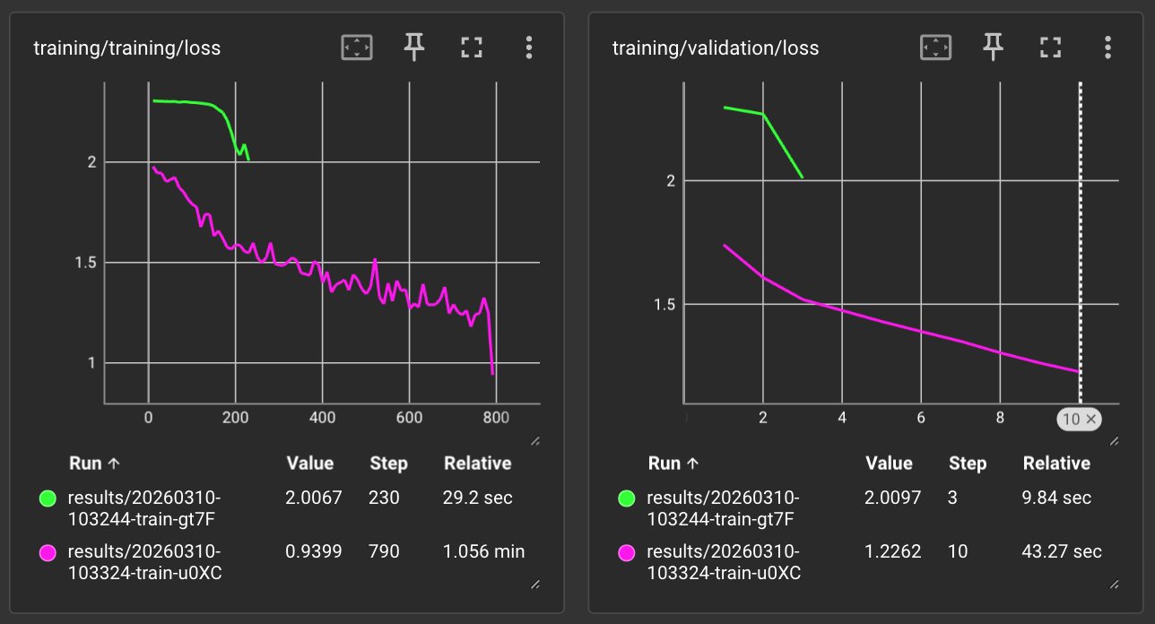
Comparing the two training runs

Using TensorBoard we can compare the loss curves side by side. The first run (green) starts from random weights and the loss decreases over 3 epochs. The second run (magenta) starts from the saved weights and immediately picks up where the first run left off, continuing to decrease over the additional epochs.

The plot on the left is the loss per batch during training, the plot on the right is the validation loss at the end of each epoch.

# Optional: load TensorBoard directly in this notebook to explore the loss curves
# %reload_ext tensorboard
# %tensorboard --logdir ./results