Extragalactic Unsupervised Discovery#
This notebook demonstrates how to run an Unsupervised Discovery workflow with a collection of HSC galaxies. It extends the shorter Astronomy Unsupervised example by adding interactive visualization of latent spaces, vector database search, and cutout inspection.
This notebook describes the full runnable science workflow:
Acquire an HSC dataset from Zenodo
Initialize and configure Hyrax
Train an autoencoder model
Run inference to produce latent representations
Reduce dimensionality with UMAP
Interactively explore the latent space with
h.visualize()Search for similar objects with a vector database
Identify anomalies using nearest-neighbour distances
The data#
This example uses roughly 1000 Hyper Suprime-Cam (HSC) cutouts, each 8 arcseconds on a side in g, i, and r bands. These cutouts were acquired previously from the HSC cutout service and cached in Zenodo for easier access.
The model#
This demonstration uses HyraxAutoencoderV2, an example model built into Hyrax. Because this is an unsupervised workflow, the goal is not classification against fixed labels, but learning a compact latent representation that can be used for similarity search and anomaly discovery.The source code for this model is available on GitHub.
[1]:
import numpy as np
import matplotlib.pyplot as plt
from pathlib import Path
Acquire an HSC dataset from Zenodo#
We acquired a small sample of HSC cutouts and cached them in Zenodo for convenience. We’ll pull those down now using pooch.
[2]:
import pooch

file_path = pooch.retrieve(
    url="doi:10.5281/zenodo.14498536/hsc_demo_data.zip",
    known_hash="md5:1be05a6b49505054de441a7262a09671",
    fname="example_hsc_new.zip",
    path="../../data",
    processor=pooch.Unzip(extract_dir="."),
)

data_dir = "../../data/hsc_8asec_1000"
Initialize Hyrax#
We begin by creating an instance of Hyrax and editing the configuration. The configuration system in Hyrax is substantial and comes with reasonable defaults. We’ll make a few changes to specify:
The model we intend to train
The number of training epochs and batch size
The data that we intend to use
The data_request defines what data each stage of the workflow should use. Here we define separate train and validation splits. You can learn more about data requests in the data requests notebook.
[ ]:
from hyrax import Hyrax

h = Hyrax()

h.set_config("model.name", "HyraxAutoencoderV2")
h.set_config("train.epochs", 20)
h.set_config("data_loader.batch_size", 32)

data_request_definition = {
    "train": {
        "data": {
            "dataset_class": "HSCDataset",
            "data_location": data_dir,
            "primary_id_field": "object_id",
        },
    },
    "validate": {
        "data": {
            "dataset_class": "HSCDataset",
            "data_location": data_dir,
            "primary_id_field": "object_id",
        },
    },
}
h.set_config("data_request", data_request_definition)
h.set_config("split", {"train": 0.8, "validate": 0.2})
Train an autoencoder model#
With the configuration set correctly, we begin training.
[ ]:
model = h.train()
The results of training are persisted by default in a timestamped directory and include:
Full copy of the complete configuration
The trained model weights
Checkpoint files
Training metric records
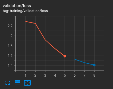
Monitoring training#
Hyrax automatically emits metrics to both TensorBoard and MLflow for real-time model performance evaluation. You can view these from the terminal or from a notebook.
For a detailed walkthrough of how to activate and use these tools, see Using TensorBoard and MLflow.
Process data with the trained model#
Now that we have a trained model, we can use it for inference to produce lower-dimensional representations of the data.
We’ll tweak the configuration before running inference to:
Increase the batch size for faster processing
Specify the data to process (in this case the same data used for training, but without splits)
[ ]:
h.config["data_loader"]["batch_size"] = 512

data_request_definition = {
    "infer": {
        "data": {
            "dataset_class": "HSCDataset",
            "data_location": data_dir,
            "primary_id_field": "object_id",
        },
    },
}
h.set_config("data_request", data_request_definition)

inference_results = h.infer()
The results are placed in a timestamped directory containing:
Inference results in Lance format
A complete copy of the configuration used
A copy of the model weights used to produce the results
You can read more about working with results in the working with results data notebook.
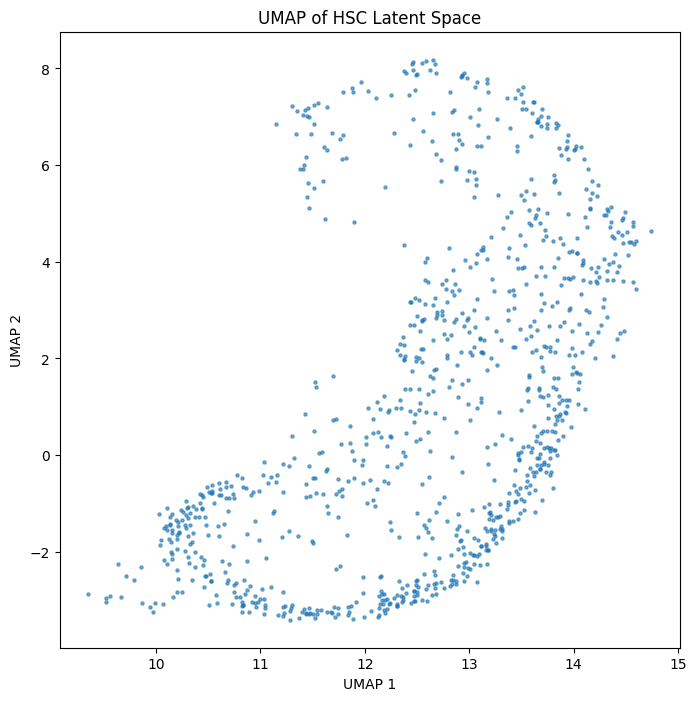
Reduce dimensionality with UMAP#
In order to visualize the latent space, we reduce its dimensionality. UMAP compresses the 64-dimensional autoencoder output down to 2 dimensions so we can plot and interact with it.
[6]:
h.set_config("reduce.umap.kwargs.n_components", 2)
h.reduce_dimensions(algorithm="umap")
[2026-06-24 17:04:27,154 hyrax.verbs.reduce_dimensions:INFO] Saving reduction results using umap to /Users/qiyuwang/Desktop/hyrax/docs/pre_executed/results/20260624-170427-umap-LNhc
[2026-06-24 17:04:27,159 hyrax.verbs.reduce_dimensions:INFO] No model_path specified. A new model will be fitted.
[2026-06-24 17:04:27,159 hyrax.verbs.reduction_algorithms.umap:INFO] Fitting the UMAP
[2026-06-24 17:04:31,013 hyrax.verbs.reduce_dimensions:INFO] Saving fitted umap reducer to result directory
[2026-06-24 17:04:32,764 hyrax.datasets.result_dataset:INFO] Optimizing Lance table after 1 batches
[2026-06-24 17:04:32,767 hyrax.datasets.result_dataset:INFO] Lance table optimization complete
[2026-06-24 17:04:32,767 hyrax.verbs.reduce_dimensions:INFO] Finished transforming all data with umap
[6]:
<hyrax.datasets.result_dataset.ResultDataset at 0x3d7e76120>
Let’s load the UMAP results and create a scatter plot of the latent space.
[7]:
from hyrax.config_utils import find_most_recent_results_dir

results_dir = str(find_most_recent_results_dir(h.config, "umap"))
data_request_definition = {
    "analysis": {
        "umap": {
            "dataset_class": "ResultDataset",
            "data_location": results_dir,
            "primary_id_field": "object_id",
        },
    }
}
h.config["data_request"] = data_request_definition
umap_results = h.prepare()
[2026-06-24 17:04:32,797 hyrax.verbs.prepare:INFO] Finished Prepare
[8]:
out = np.array([umap_results["analysis"][i]["umap"]["data"] for i in range(len(umap_results["analysis"]))])

fig, ax = plt.subplots(figsize=(8, 8))
ax.scatter(out[:, 0], out[:, 1], s=5, alpha=0.6)
ax.set_xlabel("UMAP 1")
ax.set_ylabel("UMAP 2")
ax.set_title("UMAP of HSC Latent Space")
plt.show()
Interactive visualization#
Hyrax includes a built-in interactive visualization that overlays the UMAP scatter plot with a selection table and image panel. You can lasso-select, box-select, or tap on points to inspect individual objects.
We set the filter_catalog explicitly so that the visualize verb can access HSC metadata such as RA, Dec, and filenames.
[9]:
# Set data_request back to infer with HSCDataset for the visualize verb
data_request_definition = {
    "infer": {
        "data": {
            "dataset_class": "HSCDataset",
            "data_location": data_dir,
            "primary_id_field": "object_id",
        },
    },
}
h.set_config("data_request", data_request_definition)

# Explicitly point to the manifest so the visualize verb can access metadata
h.config["data_set"]["filter_catalog"] = str(Path(data_dir).resolve() / "manifest.fits")

h.config["visualize"]["display_images"] = True
h.config["general"]["data_dir"] = data_dir
h.config["visualize"]["fields"] = ["ra_data", "dec_data"]
h.config["visualize"]["torch_tensor_bands"] = [0]
h.config["visualize"]["rasterize_plot"] = False
h.config["visualize"]["color_column"] = "ra_data"
h.config["visualize"]["cmap"] = "plasma"

viz = h.visualize(make_lupton_rgb_opts={"stretch": 8, "Q": 5}, width=550, height=550)
[2026-03-27 18:13:28,435 hyrax.verbs.visualize:INFO] UMAP directory not specified at runtime. Reading from config values.
[2026-03-27 18:13:28,517 hyrax.datasets.hsc_dataset:INFO] Checking file dimensions to determine standard cutout size...
[2026-03-27 18:13:28,519 hyrax.datasets.fits_image_dataset:INFO] FitsImageDataset has 993 objects
[2026-03-27 18:13:28,535 hyrax.datasets.hsc_dataset:INFO] Processed 993 objects for pruning
[2026-03-27 18:13:29,099 hyrax.datasets.hsc_dataset:INFO] Checking file dimensions to determine standard cutout size...
[2026-03-27 18:13:29,102 hyrax.datasets.fits_image_dataset:INFO] FitsImageDataset has 993 objects
[2026-03-27 18:13:29,118 hyrax.datasets.hsc_dataset:INFO] Processed 993 objects for pruning
[2026-03-27 18:13:29,200 hyrax.datasets.hsc_dataset:INFO] Checking file dimensions to determine standard cutout size...
[2026-03-27 18:13:29,202 hyrax.datasets.fits_image_dataset:INFO] FitsImageDataset has 993 objects
[2026-03-27 18:13:29,217 hyrax.datasets.hsc_dataset:INFO] Processed 993 objects for pruning
[2026-03-27 18:13:29,766 hyrax.verbs.visualize:INFO] Successfully loaded color values from column 'ra_data'


Calculate similarity with a vector database#
Hyrax can save inference results into a vector database for fast nearest-neighbour lookups. The Lance file format readily supports this, so for each object we can efficiently find the most similar objects in latent space.
For a dedicated walkthrough of the vector database features, see the vector database notebook.
[10]:
infer_dir = str(find_most_recent_results_dir(h.config, "infer"))
h.config["data_loader"]["batch_size"] = 512
h.save_to_database(input_dir=infer_dir)
[2026-03-27 18:13:32,454 hyrax.verbs.save_to_database:INFO] Saving vector database at /mmfs1/gscratch/dirac/aritrag/repos/hyrax/docs/pre_executed/results/20260327-181332-vector-db-6Ssf
100%|███████████████████████████████████████████████████████████████████████████████████████████████████████████████████████████████████| 2/2 [00:01<00:00,  1.34it/s]
[2026-03-27 18:13:34,154 hyrax.verbs.save_to_database:INFO] Vector database insertion complete. Total time: 0.210s for 2 batches
[11]:
vdb_dir = str(find_most_recent_results_dir(h.config, "vector-db"))
conn = h.database_connection(database_dir=vdb_dir)

object_ids = list(inference_results.ids())
search_id = object_ids[0]
nearest_neighbours = conn.search_by_id(search_id, k=10)
nn_ids = nearest_neighbours[search_id]

print(f"Query object: {search_id}")
print(f"Nearest neighbours: {nn_ids}")
Query object: 36407329666631333
Nearest neighbours: ['36407329666631333', '37481140210127257', '38554242084003517', '38553975796029667', '39613505573244081', '38549874102260404', '39613754681353146', '36424926147659595', '39618565044729823', '38544904825103196']
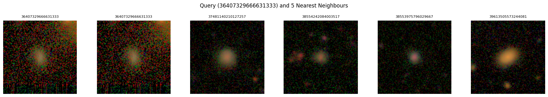
Visualize cutouts#
Let’s look at the query object alongside its nearest neighbours. Since the HSC data consists of individual FITS files per band, we load each band separately and composite them into an RGB image using astropy’s Lupton scaling.
[12]:
import glob
from astropy.io import fits
from astropy.visualization import make_lupton_rgb


def load_hsc_rgb(object_id, data_directory, bands=("HSC-I", "HSC-R", "HSC-G")):
    """Load HSC FITS cutouts and return an RGB image using Lupton scaling."""
    data_directory = Path(data_directory).expanduser().resolve()
    images = []
    for band in bands:
        pattern = str(data_directory / f"{object_id}*_{band}.fits")
        found = glob.glob(pattern)
        if not found:
            raise FileNotFoundError(f"No file matching {pattern}")
        img = fits.getdata(found[0]).astype(float)
        valid = img[~np.isnan(img)]
        if len(valid) > 0:
            img[np.isnan(img)] = np.median(valid)
        else:
            img[:] = 0
        images.append(img)
    return make_lupton_rgb(*images, Q=10, stretch=0.5)


def plot_hsc_cutouts(object_ids, data_directory, title="HSC Cutouts"):
    """Plot a row of HSC RGB cutouts for the given object IDs."""
    n = len(object_ids)
    fig, axes = plt.subplots(1, n, figsize=(3 * n, 3))
    if n == 1:
        axes = [axes]
    for ax, oid in zip(axes, object_ids):
        try:
            rgb = load_hsc_rgb(str(oid), data_directory)
            ax.imshow(rgb, origin="lower")
        except Exception as e:
            ax.text(
                0.5,
                0.5,
                f"Error:\n{e}",
                ha="center",
                va="center",
                transform=ax.transAxes,
                fontsize=7,
                color="red",
            )
        ax.set_title(f"{oid}", fontsize=8)
        ax.axis("off")
    fig.suptitle(title, fontsize=12, y=1.02)
    plt.tight_layout()
    plt.show()
    return fig, axes
[13]:
# Plot the query object and its 5 nearest neighbours side by side
plot_hsc_cutouts([search_id] + nn_ids[:5], data_dir, title=f"Query ({search_id}) and 5 Nearest Neighbours")
[13]:
(<Figure size 1800x300 with 6 Axes>,
 array([<Axes: title={'center': '36407329666631333'}>,
        <Axes: title={'center': '36407329666631333'}>,
        <Axes: title={'center': '37481140210127257'}>,
        <Axes: title={'center': '38554242084003517'}>,
        <Axes: title={'center': '38553975796029667'}>,
        <Axes: title={'center': '39613505573244081'}>], dtype=object))
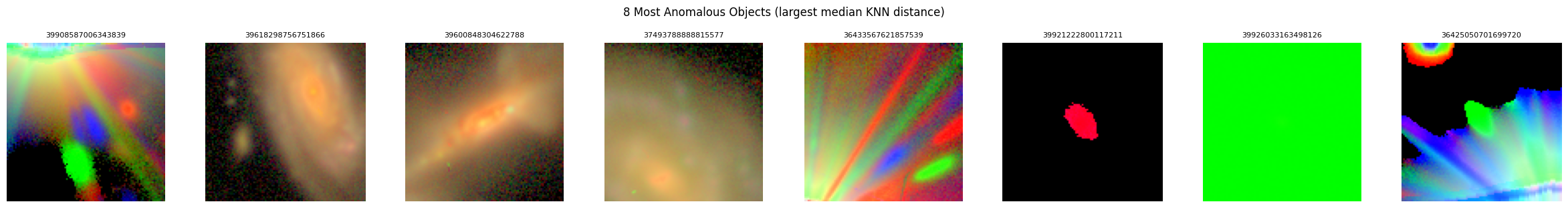
Identify anomalies with nearest-neighbour distances#
For each object, we find the L2 distances to its 5 nearest neighbours in the latent space. The median of those distances gives a single “outlier score” per object.
Objects with unusually large median distances live far from any cluster in the latent space, making them candidates for anomalies — artifacts, rare morphologies, or blended sources.
[14]:
all_embeddings = [inference_results[i].flatten() for i in range(len(inference_results))]

knn_distances = []
for emb in all_embeddings:
    results = inference_results.table.search(emb).metric("L2").limit(6).to_list()
    dists = [r["_distance"] for r in results[1:]]  # skip self
    knn_distances.append(dists)

median_dist = np.median(knn_distances, axis=1)

plt.figure(figsize=(8, 4))
plt.hist(median_dist, bins=100, range=(0, np.mean(median_dist) * 2))
plt.xlabel("Median L2 distance to k=5 nearest neighbours")
plt.ylabel("Count")
plt.title("Distribution of KNN distances")
plt.show()
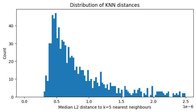
There appears to be a long tail in the distribution, indicating that a small number of objects have latent representations that are far from any cluster. Let’s compare the most “normal” objects (smallest median distance) with the most “anomalous” (largest median distance).
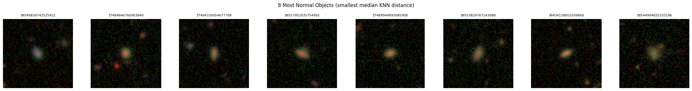
[15]:
sorted_indices = np.argsort(median_dist)
normal_ids = [object_ids[i] for i in sorted_indices[:8]]
anomalous_ids = [object_ids[i] for i in sorted_indices[-8:]]

plot_hsc_cutouts(normal_ids, data_dir, title="8 Most Normal Objects (smallest median KNN distance)")
plot_hsc_cutouts(anomalous_ids, data_dir, title="8 Most Anomalous Objects (largest median KNN distance)")
[15]:
(<Figure size 2400x300 with 8 Axes>,
 array([<Axes: title={'center': '39908587006343839'}>,
        <Axes: title={'center': '39618298756751866'}>,
        <Axes: title={'center': '39600848304622788'}>,
        <Axes: title={'center': '37493788888815577'}>,
        <Axes: title={'center': '36433567621857539'}>,
        <Axes: title={'center': '39921222800117211'}>,
        <Axes: title={'center': '39926033163498126'}>,
        <Axes: title={'center': '36425050701699720'}>], dtype=object))
The “normal” objects tend to be compact and isolated, while the “anomalous” objects tend to be extended, in crowded fields, or contain instrument artifacts.
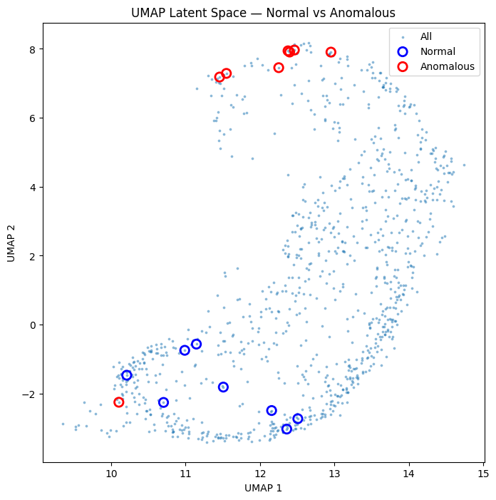
We can overlay these two populations on the UMAP scatter plot to see how they separate in the latent space.
[16]:
normal_umap = out[sorted_indices[:8]]
anomalous_umap = out[sorted_indices[-8:]]

fig, ax = plt.subplots(figsize=(8, 8))
ax.scatter(out[:, 0], out[:, 1], s=3, alpha=0.4, label="All")
ax.scatter(
    normal_umap[:, 0],
    normal_umap[:, 1],
    s=80,
    edgecolor="blue",
    facecolor="none",
    linewidths=2,
    label="Normal",
)
ax.scatter(
    anomalous_umap[:, 0],
    anomalous_umap[:, 1],
    s=80,
    edgecolor="red",
    facecolor="none",
    linewidths=2,
    label="Anomalous",
)
ax.set_xlabel("UMAP 1")
ax.set_ylabel("UMAP 2")
ax.set_title("UMAP Latent Space — Normal vs Anomalous")
ax.legend()
plt.show()
What to take away#
The full Hyrax pipeline — from data acquisition through anomaly discovery — can be driven entirely from a notebook with a handful of configuration calls and verbs.
Vector databases enable fast similarity search over the latent space. Hyrax stores inference results in Lance format, which supports efficient nearest-neighbour queries out of the box.
Interactive visualization with
h.visualize()lets you lasso-select, tap, and inspect objects directly in the UMAP scatter plot.KNN distance is a simple but effective anomaly score. The long tail of the distance histogram highlights objects that the model finds unusual.
Possible next steps:
Perform clustering to search for additional sub-populations
Filter out instrument artifacts and re-train
Swap in a different model (e.g.
ImageDCAEor your own custom model)Use hyperparameter tuning to optimize model performance
[ ]: